Algebraic structure of musical intervals and pitches

Here’s the first in what will hopefully be a series of related posts about one particular (limited) aspect of the interaction between music and mathematics. In my mind, I’ll be explaining things to a hypothetical musically uneducated mathematician, who should nevertheless end up with an understanding as good as any bona-fide musician’s – in the tradition of certain physics books of which I am a fan.

I begin by revising, in unnecessary rigorous detail, what you already knew about musical pitches and intervals.

Musical intervals are the signed distance between musical notes, as written on a traditional (Western) five-lined musical stave. For completeness, I will first summarise traditional pitch and interval notation.

Pitch syntax

Pitches are a pair, consisting of a letter and an accidental: $P = (N, a)$ , $P \in \mathcal{P}$ , where

$N \in \{A,B,C,\ldots,A',\ldots\}, \\ a \in \{\natural,\sharp,\flat,\sharp\sharp,\flat\flat,\ldots,\sharp^n,\flat^n,\ldots\}$

leading to constructions such as C♮, F♯, B♭ etc. These pitches correspond in a slightly irregular way to the horizontal lines (and gaps between them) on the stave, but I will not go into the details here. All pairs $(N, a)$ correspond to valid pitches. The set of pitches is actually extended upwards beyond that written above with super-prime symbols ( $A', B'$ ), and downwards with sub-primes ( $C_{'},D_{'}$ ).

The accidentals are pronounced as follows: ♮ is a natural, ♭ is a flat, ♯ is a sharp.

Pitches form an affine space, with intervals as the difference type (subtraction of two pitches). I will not define this subtraction until we have a clearer idea of the algebra of intervals.

Interval syntax

Intervals are also a pair, consisting of a quality and a number: $I = (q, n)$ , $I \in \mathcal{I}$ , where

$q \in \{\mathsf{P,M,m,A,d,AA,dd},\ldots,\mathsf{A}^n,\mathsf{d}^n,\ldots\}, \\ n \in \{\ldots,\mathsf{-3,-2,1,2,3},\ldots\}$

leading to interval names such as P5, M3, m6 etc. Note that the set which $n$ belongs to is not ℤ – the $n$ are simply an arbitrary label (nominal numbers), and their arithmetic is tied up with the overall algebra of musical intervals in a complex way that does not correspond to the conventional notion of integers. Intervals form an associative abelian algebra (generally written as addition), together with the four additional operations of augmentation, diminution, inversion and negation.

The interval qualities listed above are pronounced, respectively, perfect, major, minor, augmented, diminished, doubly augmented etc. The interval numbers are pronounced as ordinal numbers, with the special case that $8$ is an octave, and $1$ a unison.

Note also that not all combinations $(q, n)$ are permitted; in particular, there are certain rules that allow one to construct valid intervals. Start with one of the eleven valid base intervals:

$\mathcal{I}' = \{\mathsf{P1}, \mathsf{m2}, \mathsf{M2}, \mathsf{m3}, \mathsf{M3}, \mathsf{P4}, \mathsf{P5}, \mathsf{m6}, \mathsf{M6}, \mathsf{m7}, \mathsf{M7}\}.$

The total set $\mathcal{I}$ of valid intervals is actually periodic: take $\mathcal{I}'$ , and in the positive $n$ direction $\mathcal{I}$ has period 7 and the entire inverted set (the result of the map $n \longrightarrow -n$ ) is also in $\mathcal{I}$ , i.e.

$(q,n) \in \mathcal{I}' \implies (q,n \pm 7m) \in \mathcal{I}^{\prime\prime},$

and then also

$(q,n) \in \mathcal{I}^{\prime\prime} \implies (q, -n) \in \mathcal{I} \:\: \mathrm{and} \:\: (q, n) \in \mathcal{I}.$

Operations on intervals

I will freely interchange two forms of notation for the same interval: $\mathsf{P5}$ and $(P,5)$ for convenience. I will use $+$ for interval vector addition and addition of intervals to pitches, and $-$ for interval vector subtraction and subtraction of pitches. I will use a dot $\cdot$ for scalar multiplication of interval vectors by integers.

Before I get to the complete decision procedure for intervallic addition below, a limited form of interval addition can be defined on $\mathcal{I}'$ ,

$\mathsf{P1} + I = I\\ (\mathsf{M},n) - (m,n) = \mathsf{m2}\\ (\mathsf{m},n+1) - (\mathsf{M},n) = \mathsf{m2}\\ (\mathsf{m},n+1) - (\mathsf{P},n) = \mathsf{m2},\\$

which can be extended in the obvious way to $\mathcal{I}$ (of course, each case is defined only for $(q,n)$ that actually exist in $\mathcal{I}$ ).

Then, you can augment intervals:

$aug(q,n) = \begin{cases} (\mathsf{A},n) & \mbox{if } q = \mathsf{P} \\ (\mathsf{M},n) & \mbox{if } q = \mathsf{m} \\ (\mathsf{A},n) & \mbox{if } q = \mathsf{M} \\ (\mathsf{m},n) & \mbox{if } q = \mathsf{d} \mbox{ and } (\mathsf{m},n) \in \mathcal{I} \\ (\mathsf{P},n) & \mbox{if } q = \mathsf{d} \mbox{ and } (\mathsf{P},n) \in \mathcal{I} \\ (\mathsf{A}^{i+1},n) & \mbox{if } q = \mathsf{A}^i \\ (\mathsf{d}^{i-1},n) & \mbox{if } q = \mathsf{d}^i,\\ \end{cases}$

and diminish them:

$dim(q,n) = \begin{cases} (\mathsf{d},n) & \mbox{if } q = \mathsf{P} \\ (\mathsf{m},n) & \mbox{if } q = \mathsf{M} \\ (\mathsf{d},n) & \mbox{if } q = \mathsf{M} \\ (\mathsf{M},n) & \mbox{if } q = \mathsf{A} \mbox{ and } (\mathsf{M},n) \in \mathcal{I} \\ (\mathsf{P},n) & \mbox{if } q = \mathsf{A} \mbox{ and } (\mathsf{P},n) \in \mathcal{I} \\ (\mathsf{A}^{i-1},n) & \mbox{if } q = \mathsf{A}^i.\\ (\mathsf{d}^{i+1},n) & \mbox{if } q = \mathsf{d}^i \\ \end{cases}$

Note that $aug(dim(I)) = dim(aug(I)) = I$ , for all $I$ .

We can now define addition on intervals. Let $I_1 = (q_1,n_1)$ and $I_2 = (q_2,n_2)$ . Then,

$I_1 + I_2 = I_3 = (q_3, n_3),$

finding $q_3$ and $n_3$ according to the following procedure: augment or diminish $I_1$ until you have a new interval $I'_1 \in \mathcal{I}$ , along the way calculating an augmentation index $j_1$ , where you increment $j_1$ once for each augmentation, and decrement once for each diminution. Repeat for $I'_2$ . Then perform the following interval addition, which is possible because addition is already defined on $\mathcal{I}$ :

$I'_1 + I'_2 = I'_3.$

Then, perform the appropriate number ( $j_1 + j_2$ ) of augmentations on $I'_3$ , to give $I_3$ :

$aug^{j_1+j_2}(I'_3) = (q_3,n_3).$

Incidentally, it is always true that $n_3 = n_1 + n_2 - 1$ .

Free abelian groups

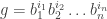
Quick revision of free abelian groups. A free abelian group $G$ of rank $n$ satisfies the following: there exists at least one set $B \subset G$ , with $|B| = n$ , such that every element of $G$ can be written as a linear combination of the elements of $B$ , with integer coefficients, i.e. $g = b_1^{i_1}b_2^{i_2}\ldots b_n^{i_n}$ .

Free abelian groups can be thought of as vector spaces over the integers (ℤ as the field of scalars, $G$ as the group of vectors).

A rank- $n$ free abelian group is isomorphic to the group of $n$ -tuples of integers, with the group operation pairwise addition:

$(a_1,a_2,\ldots) + (b_1,b_2,\ldots) = (a_1 + b_1, a_2 + b_2, \ldots),$

or in other words, any rank- $n$ free abelian group is isomorphic to the direct sum of $n$ copies of ℤ:

$G \cong \mathbb{Z} \oplus \mathbb{Z} \oplus \ldots \oplus \mathbb{Z}.$

There may be many different choices of basis set $b$ , much like a vector space with no preferred basis.

Intervals as a free abelian group

As you can probably tell, our previous method of interval addition is a horrible mess. Luckily we can prove that intervals form a rank-2 free abelian group (said proof consists of a pile of tedious case analysis). Hence we can find a two-element basis; after which interval addition proceeds easily, being reduced to element-wise addition of pairs of integers.

We need to find any pair of linearly independent intervals to use as a basis – to decompose any arbitrary interval into a linear combination of the two basis intervals. Once we have one basis, we can use them to easily generate all the other bases. However, it’s not immediately obvious how to find our first pair of linearly independent intervals. Luckily, I have such a pair up my sleeve already: (A1, d2). They must be linearly independent, because

$n\cdot \mathsf{A1} = (\mathsf{A}^n, n - n + 1) = (\mathsf{A}^n,1) \neq \mathsf{d2} \:\:\: \forall n.$

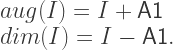
We will now take the opportunity to simplify our augmentation and diminution operations,

$aug(I) = I + \mathsf{A1} \\ dim(I) = I - \mathsf{A1}.$

Decomposing arbitrary intervals into a basis requires some more tedious case analysis, so here are just a few examples:

$\mathsf{m2} = \mathsf{A1} + \mathsf{d2}\\ \mathsf{P5} = 7\cdot \mathsf{A1} + 4\cdot \mathsf{d2}\\ \mathsf{M6} = 9\cdot \mathsf{A1} + 5\cdot \mathsf{d2}\\ \mathsf{P8} = 12\cdot \mathsf{A1} + 7\cdot \mathsf{d2}.$

If we define the map $\phi : \mathcal{I} \longrightarrow \mathbb{Z}\times\mathbb{Z}$ to be the map that gives the decomposition into the (A1, d2) basis, then the above could be written as

$\phi(\mathsf{m2}) = (1,1)\\ \phi(\mathsf{P5}) = (7,4)\\ \phi(\mathsf{M6}) = (9,5)\\ \phi(\mathsf{P8}) = (12,7).$

The basis (A1, d2) is convenient insofar as A1 matches up with what we think of as semitones, and d2 simply counts an interval’s number.

Now that we can add and subtract intervals easily, I can concisely define the two remaining special operations on intervals, inversion and negation:

$inv(I) = \mathsf{P8} - I\\ neg(I) = \mathsf{P1} - I.$

Pitch space

Of course, merely being able to add and subtract intervals is pretty useless on its own. What we really want to do is use intervals to hop around the space of pitches. The rules for pitch arithmetic are only barely less irregular than for intervals.

Note: adding an interval to a pitch is called transposition, and it is technically a separate operation from interval addition (it has a different type signature), but we shall use the $+$ symbol for it anyway.

In our notation from the first section, adding an octave (P8) adds a prime symbol to a letter name

$(N,a) + \mathsf{P8} = (N',a)\\ (N_{'},a) + \mathsf{P8} = (N,a)$

with the obvious extension to multiple octave subtraction, and multiple primes and sub-primes.

Adding and subtracting A1 corresponds to adding and subtracting sharps and flats:

$(N,\natural) + \mathsf{A1} = (N,\sharp)\\ (N,\flat) + \mathsf{A1} = (N,\natural)$

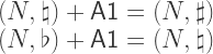
with the obvious extension to double sharps (♯♯) and double flats (♭♭) and arbitrary numbers of accidentals.

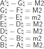
All that remains is to give the intervals between the natural (♮) pitches:

$\mathsf{A'\natural} - \mathsf{G\natural} = \mathsf{M2}\\ \mathsf{G\natural} - \mathsf{F\natural} = \mathsf{M2}\\ \mathsf{F\natural} - \mathsf{E\natural} = \mathsf{m2}\\ \mathsf{E\natural} - \mathsf{D\natural} = \mathsf{M2}\\ \mathsf{D\natural} - \mathsf{C\natural} = \mathsf{M2}\\ \mathsf{C\natural} - \mathsf{B\natural} = \mathsf{m2}\\ \mathsf{B\natural} - \mathsf{A\natural} = \mathsf{M2}.$

The equivalent of choosing a basis for our intervals is finding a coordinate system for our pitches. To do this we must convert the pitch affine space $\mathcal{P}$ into a vector space (Wikipedia suggests the name Pointed space) by choosing an origin. At this point, any choice of origin is arbitrary and meaningless, but it becomes important when we get to tuning systems, which will be the subject of the next post in this series.

For example, let us define a map $\psi : \mathcal{P} \longrightarrow \mathbb{Z}\times\mathbb{Z}$ with origin

$\psi(\mathsf{A\natural}) = O.$

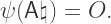
Then, to find the coordinates of an arbitrary pitch $P$ , we compute

$\psi(P) = O + \phi(P - O).$

Of course, it is easiest to simply define $O = (0,0)$ .

We now no longer need to worry about how to represent pitches, and will focus on intervals for the purposes of basis changes.

Change of interval basis

Given that we now have one valid basis, the problem of further changes of basis reduces to linear algebra in two dimensions.

Let $\phi(I) = (m,n)$ be our interval in the (A1,d2) representation, and let $\phi(I_1) = (a,b)$ and $\phi(I_2) = (c,d)$ be a different pair of linearly independent basis intervals. Then

$x\cdot(a,b) + y\cdot(c,d) = (m,n),$

which is simply a system of two linear equations, to be solved by determinants in the usual way:

$x = \frac{dm - cn}{ad - bc}, \:\:\:\: y = \frac{an - bm}{ad - bc}.$

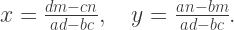
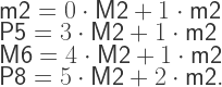
Clearly the solution will not always be in the integers, so we may sometimes choose to extend our scalar field to the rationals (particularly when we come to tuning systems). Here are the examples from the previous-but-one section, but demonstrating the (P5,P8) basis:

$\mathsf{m2} = -5\cdot\mathsf{P5} + 3\cdot\mathsf{P8}\\ \mathsf{P5} = 1\cdot\mathsf{P5} + 0\cdot \mathsf{P8}\\ \mathsf{M6} = 3\cdot \mathsf{P5} - 1\cdot\mathsf{P8}\\ \mathsf{P8} = 0\cdot \mathsf{P5} + 1\cdot\mathsf{P8},$

and again with the (M2,m2) basis:

$\mathsf{m2} = 0\cdot\mathsf{M2} + 1\cdot\mathsf{m2}\\ \mathsf{P5} = 3\cdot\mathsf{M2} + 1\cdot\mathsf{m2}\\ \mathsf{M6} = 4\cdot \mathsf{M2} + 1\cdot\mathsf{m2}\\ \mathsf{P8} = 5\cdot \mathsf{M2} + 2\cdot \mathsf{m2}.$

Finally, here is a diagram showing pitch space, with arrows representing 3 choices of interval basis.

Figure 1: Lattice

The ideas in this post are implemented concretely in two software projects: the Haskell Music Suite (also available on Hackage), and in AbstractMusic (the latter being my own personal research project).