There’s a wide class of coordinate transforms that are typically given backwards. Witness spherical polar coordinates:
Typically we already know what our cartesian coordinates 


but it looks like we’ve only been given the inverse map

Now, really we know how to invert these expressions. But doing calculus with inverse functions like 
What we’re interested in is what becomes of the basis vectors 

Let’s imagine that the manifold 


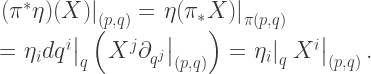
Recall that a map 


But this is exactly the same as saying that the pullback induced by the inverse map 

Another way of phrasing this is that the exterior derivative commutes with pullbacks. Let 


A correct method for covectors
But now let 


using the fact that we know 

Rinse and repeat for the other basis covectors:

So given a covector 


An incorrect method for vectors
But what about ordinary vectors?
Let’s try and naively apply the calculus we already know, so try the following (for the 

Now when we contract this with our earlier expression for 
But instead we get

What went wrong? We neglected to consider contributions to 
A correct method for vectors
Write out completely general expressions for

All we know about these basis vectors is that, when contracted with the basis covectors, we should obtain the identity matrix, even when they’ve been written out in spherical coordinates:
(
So we repeatedly apply this property to the expression above, essentially inverting the 3-by-3 matrix that has components 
For example, for

which gives the correct result when contracted with
Conclusion
The essential difference between vectors and covectors is that, under maps, one of them moves one way and the other one moves the other way. Hopefully the little parable in this blogpost has illustrated this fact.
When you have a metric you can talk about them having indices in different places, but that allows you to forget about the difference between them altogether! The interesting differences between vectors and covectors come into play when:
- You don’t necessarily know what the metric is.
- You’re using maps between manifolds/coordinate systems whose inverses don’t necessarily exist (for example, the projection onto a submanifold has no inverse).
The fact that the exterior derivative commutes with pullbacks also explains why it’s covectors that show up in integrals, thanks to the ‘change of variables’ formula

It also explains why it’s so easy to find the form of the metric in new coordinates, because the metric is a rank (0,2)-tensor, i.e. a sum of pairs of covectors, tensor-producted together:

and we can just substitute for 
 ) which is supposedly key to the whole process. Here I will attempt to describe what this 1-form is, why it is useful, and the role it plays in the fundamentals of classical mechanics.
  be a smooth function, let
  be a vector field on
  be a covector field on


 ) and a vector field (a function
  ), and similarly for covectors. Typically, the various kinds of product are evaluated pointwise, e.g. if
  are functions then
  .
.  be a smooth manifold, and specialise the above discussion to the case
  ,
,  . Let
. Let  be coordinates on
  be coordinates on
  ; that is, points on
  . Having these two equivalent ways to look at points on a cotangent bundle is an important point which we shall return to later.
 interpreted as a 1-form, and also has the coordinate expression
  . How on earth can both these things be true, and besides, how can one ‘interpret a pullback as a 1-form’?!
  induces a pullback
  , but this map has exactly the domain and range of a covector field on
  as a coordinate on
  for coordinates on
  , equivalently writing
  where in a slight abuse of notation we’ve written
  for the first
  coordinates (the
  components) and
  for the second
  components).
  and its induced pullbacks and pushforwards. Let
  be a function on
 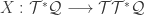 be a vector field on
  .
.  , the pushforward of
  under
under 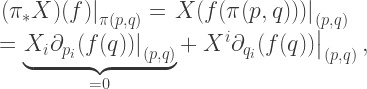
 are
are  , i.e. just the
  (in coordinates
  ):
): 
 is basically to place

 . Treating
  as a map (a similar trick to above) means it induces a pushforward
  and a pullback
  .
.  be a function, and
  a vector field with coordinate expression
  , which is pushed-forward like so:
 acts on covector fields
  :
: 
 , the interesting 1-form we were looking at above? We get
 that satisfies various properties; notably that
  , so that at least locally we can find an
  . Abstractly, we want to find paths
  such that the action integral
  is minimised:
 (the minus sign being a mere convention) where
  that takes curves
  and gives a real number, and they would then find the curve
  that minimises that number (
![\gamma : [0,1] \longrightarrow \mathcal{Q}](https://s0.wp.com/latex.php?latex=%5Cgamma+%3A+%5B0%2C1%5D+%5Clongrightarrow+%5Cmathcal%7BQ%7D&bg=ffffff&fg=333333&s=0&c=20201002) .
.  be a class of curves in
  and ending point
  . Now define
 ![W(q) \equiv S[\gamma_q] + W_0](https://s0.wp.com/latex.php?latex=W%28q%29+%5Cequiv+S%5B%5Cgamma_q%5D+%2B+W_0&bg=ffffff&fg=333333&s=0&c=20201002) for some constant
for some constant  , where
  that minimises
 ![S[\gamma_q]](https://s0.wp.com/latex.php?latex=S%5B%5Cgamma_q%5D&bg=ffffff&fg=333333&s=0&c=20201002) . This function
. This function  is called Hamilton’s principal function, and note that it depends only on positions, and not the momenta! We now calculate
 ![S[\gamma_q] = W(q) - W(q_0) \\ \:\:\:\: = \int_{\partial \gamma_q} W \\ \ \:\:\:\: = \int_{\gamma_q} dW \:\:\:\:\:\:\:\: (1) \\ \ \:\:\:\: = \int_{\gamma_q} (dW)^* \theta \:\:\:\:\:\:\:\: (2) \\ \ \:\:\:\: = \int_{dW(\gamma_q)} \theta \:\:\:\:\:\:\:\: (3) \\ \ \:\:\:\: = \int_\Gamma \theta.](https://s0.wp.com/latex.php?latex=S%5B%5Cgamma_q%5D+%3D+W%28q%29+-+W%28q_0%29+%5C%5C+%5C%3A%5C%3A%5C%3A%5C%3A+%3D+%5Cint_%7B%5Cpartial+%5Cgamma_q%7D+W+%5C%5C+%5C+%5C%3A%5C%3A%5C%3A%5C%3A+%3D+%5Cint_%7B%5Cgamma_q%7D+dW+%5C%3A%5C%3A%5C%3A%5C%3A%5C%3A%5C%3A%5C%3A%5C%3A+%281%29+%5C%5C+%5C+%5C%3A%5C%3A%5C%3A%5C%3A+%3D+%5Cint_%7B%5Cgamma_q%7D+%28dW%29%5E%2A+%5Ctheta+%5C%3A%5C%3A%5C%3A%5C%3A%5C%3A%5C%3A%5C%3A%5C%3A+%282%29+%5C%5C+%5C+%5C%3A%5C%3A%5C%3A%5C%3A+%3D+%5Cint_%7BdW%28%5Cgamma_q%29%7D+%5Ctheta+%5C%3A%5C%3A%5C%3A%5C%3A%5C%3A%5C%3A%5C%3A%5C%3A+%283%29+%5C%5C+%5C+%5C%3A%5C%3A%5C%3A%5C%3A+%3D+%5Cint_%5CGamma+%5Ctheta.+&bg=ffffff&fg=333333&s=2&c=20201002)


 as a pullback, similarly to the trick we pulled above with
 , and call it time
  , and similarly one of the momenta, say
  , and call it energy
  (again, minus sign by convention), so that
 in favour of the other coordinates (we will still write
  and
and  for the other (n-1) coordinates).
  by the definition of the exterior derivative, so we can immediately write down the first of Hamilton’s equations:
 property, we can define a quantity that gives us the second of Hamilton’s equations:


![S[\gamma] = \int_\gamma \left.g(X,X)\right|_{\gamma(s)}ds](https://s0.wp.com/latex.php?latex=S%5B%5Cgamma%5D+%3D+%5Cint_%5Cgamma+%5Cleft.g%28X%2CX%29%5Cright%7C_%7B%5Cgamma%28s%29%7Dds+&bg=ffffff&fg=333333&s=2&c=20201002)
 is arc length,
  the metric, and
  . The associated time-agnostic (‘non-autonomous’) method is fairly difficult, and this article discusses all the details.
 of a manifold
  ; relevant observables can be functions of both position and momentum. For example, the distribution function
  , which is the number density of particles in phase space (
 and
and  are coordinates on
  respectively).
  , where
  is the determinant of the metric evaluated at
  ; and the volume form for the full phase space is
  . If we want to integrate out the momentum-dependence of some observable, we need just the momentum-part of the volume form. From the two expressions above we can see that this is
  .
.  , given by
 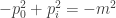 , where
  .
.  , and note that the equation for
 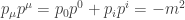 , which allows us to solve for
 . Noting that the metric is a function of
 are covariant to begin with).

 with respect to a spatial component
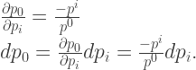
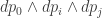 can be simplified to involve only the
  -component of
  (
(  ), as repetition of a form in a wedge product sets the entire expression to zero. We also have
  .
. 


 does not appear in the final volume form, so we are free to set
  if we choose, as is the case with photons.
  , containing
  (~millions) points
  . Perhaps it’s the output of an
  – for example
  , the mass at each point.
  , and calculate some function at every point within it. For example, approximate the integral of the density by summing over the mass at each point:
 , where
  ,
,  contains only zeroes or ones, and
  contains
  iff
iff  ; also
  , but
, but  . Assume that this operation can be calculated efficiently (in parallel), as opposed to sequentially traversing the elements of an array, which is much slower (this is the case in the IDL programming language, for example).
  at each point – that is,
  if
if  and
and  otherwise. Then the final calculation is
 is itself a very large set, and that we have another, smaller region
  on which we would also like to perform calculations. Let
  and
and  . Then we can compose our masks to find the
  values that lie within
  .
. 
![\displaystyle A = [0,1,2,\ldots,|S|] \\ B = (A \star S) \star S'](https://s0.wp.com/latex.php?latex=%5Cdisplaystyle++A+%3D+%5B0%2C1%2C2%2C%5Cldots%2C%7CS%7C%5D+%5C%5C+B+%3D+%28A+%5Cstar+S%29+%5Cstar+S%27+&bg=ffffff&fg=333333&s=0&c=20201002)
 is written as
 , i.e. a map that takes intervals to pitch ratios. We fix two intervals,
  and
and  . Assuming it is not the case that
  , these two intervals span
  , so
, so  is now fixed for all
  . This is because any
  basis,

 , otherwise octaves aren’t pure!
  (e.g. P5) can be specified freely; then, perhaps
  (e.g. P4) will come out correct too. After that you’re out of luck.
  for the perfect fifth, and
  for the octave. As indicated above, this completely specifies the tuning. The procedure for general intervals is then as follows:


 , i.e.
  for some note
  ; the common choice is
  , and
, and 


 :
: 


 .
.  , and note-mapping
  .
.  ), assign the notes
  to their keys (with frequencies
  ), ending at
  (
( depending on whether
  . This is called a wolf interval, and its existence limits the usefulness of syntonic tuning systems for keyboards.
  : under Pythagorean tuning, the A3 is about
  , to contrast with the pure P4 which is exactly
  .
.  for some interval
  , and use
  as our new basis, then because
  for some rational
  carefully so that all intervals can actually be represented by
  , then the tuning system is called


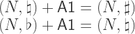
 and
and  . This means that
  , and
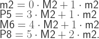
, and  . So A1 and m2 are identified, and are used as the generator
  , which is extremely close to the Pythagorean value!
  , and five “black” notes
  . There are no more notes to account for, because the equivalency of A1 and m2 means that notes that differ by these intervals are identified, e.g.
  and
and  .
.  .
. 
 be a curve on
  in some coordinate system, and
  in some other coordinate system. Then we can find a ‘velocity’ vector
  , tangent to the curve, whose coordinates are
  . The coordinates of
 with a basis by pairing up its components
  with a basis
  , as well as the same in the primed coordinate system:
 for short – imagine a flat plane (
  ; in this case we can just say that it lives in
  , and we have to be careful not to forget about its position-dependence even if we suppress it occasionally for notational convenience.
  be a scalar field (just a real-valued function) on our manifold
 . The
. The 
 as components of a vector, we’ve found a one-to-one correspondence between vectors and first-order differential operators (strictly speaking it’s between vector components and operators, but all the transformation matrices between coordinate systems are one-to-one too so it doesn’t matter).
  certainly transform in the correct way. We now make the formal identification
 and
and  when talking about operators; and
  and
and  when talking about basis vectors.
  that satisfies linearity, i.e.
 , rather than the
 must be coordinate independent, as the left hand side makes no reference to any coordinate system; and we already know how to transform
  must use the opposite transformation,
  . So we have

 , much like how we earlier decided that
  .
. 
 , which we have defined to be true.
  now comes in handy as a way to generate new covectors. In fact, covectors generated in this way have the following useful property:
 will not be the differential of any function at all.


 . Unfortunately you also see people write the above as
 ,
,  , where
 correspond to valid pitches. The set of pitches is actually extended upwards beyond that written above with super-prime symbols (
 ), and downwards with sub-primes (
 ).
).  ,
,  , where
 is an octave, and
  a unison.
  are permitted; in particular, there are certain rules that allow one to construct valid intervals. Start with one of the eleven valid base intervals:
 , and in the positive
  ) is also in

 and
and  for convenience. I will use
  for interval vector addition and addition of intervals to pitches, and
  for interval vector subtraction and subtraction of pitches. I will use a dot
  for scalar multiplication of interval vectors by integers.
 that actually exist in

 , for all
  and
and  . Then,
 and
and  according to the following procedure: augment or diminish
  until you have a new interval
  , along the way calculating an augmentation index
  , where you increment
  . Then perform the following interval addition, which is possible because addition is already defined on
 ) of augmentations on
  , to give
  :
: 
 .
.  of rank
  , with
  , such that every element of
  .
. 


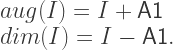

 to be the map that gives the decomposition into the (A1, d2) basis, then the above could be written as


 into a vector space (Wikipedia suggests the name
  with origin

 .
.  be our interval in the (A1,d2) representation, and let
  and
and  be a different pair of linearly independent basis intervals. Then