Implicit coordinate transforms are weird

There’s a wide class of coordinate transforms that are typically given backwards. Witness spherical polar coordinates:

$x = r \cos \phi \sin \theta \\ y = r \sin \phi \sin \theta \\ z = r \cos \theta \\$

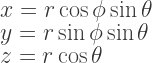
Typically we already know what our cartesian coordinates $(x,y,z)$ are, and we want to express them in this fancy new coordinate system $(r,\phi,\theta)$ . That is, we want a map

$\Phi : (x, y, z) \mapsto (r, \phi, \theta),$

but it looks like we’ve only been given the inverse map

$\Phi^{-1} : (r, \phi, \theta) \mapsto (x, y, z) = (r \cos \phi \sin \theta, r \sin \phi \sin \theta, r \cos \theta).$

Now, really we know how to invert these expressions. But doing calculus with inverse functions like $\tan^{-1}(y/x)$ is no fun at all, and besides we can imagine situations where no inverse exists.

What we’re interested in is what becomes of the basis vectors $(\partial_x, \partial_y, \partial_z)$ and covectors $(dx, dy, dz)$ when we change to spherical polar coordinates.

Let’s imagine that the manifold $\mathcal{M}$ is “ $\mathbb{R}^3$ with cartesian lines drawn on”, and the manifold $\mathcal{N}$ is “ $\mathbb{R}^3$ with spherical lines drawn on”. Obviously these are both $\mathbb{R}^3$ , but our reasoning will be completely general.

Recall that a map $\Phi : \mathcal{M} \longrightarrow \mathcal{N}$ induces a ‘pullback’ $\Phi^*$ that takes functions/covectors on $\mathcal{N}$ to functions/covectors on $\mathcal{M}$ ; and a ‘pushforward’ $\Phi_*$ that takes curves/vectors on $\mathcal{M}$ to curves/vectors on $\mathcal{N}$ . That is, the pullback $\Phi^*$ operates ‘backwards’ to the direction of the original map $\Phi$ .

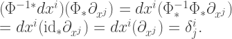
But this is exactly the same as saying that the pullback induced by the inverse map $\Phi^{-1}$ will operate in the expected ‘forwards’ direction. So, $\Phi^{-1*}$ takes functions/covectors on $\mathcal{M}$ to functions/covectors on $\mathcal{N}$ . So, given that we only have access to $\Phi^{-1}$ right now, it looks like we can successfully work out what our covectors will look like in spherical coordinates.

Another way of phrasing this is that the exterior derivative commutes with pullbacks. Let $f$ be a function on $\mathcal{M}$ and $v$ a vector field on $\mathcal{N}$ . Then

$(\Phi^{-1*} df)(v) = df(\Phi^{-1}_*v) = (\Phi^{-1}_*v)(f) \\ = v(\Phi^{-1*}f) = d(\Phi^{-1*}f)(v) \\ \Rightarrow \Phi^{-1*}df = d(\Phi^{-1*}f).$

A correct method for covectors

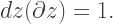
But now let $f$ be the coordinate function for the coordinate $x$ , i.e. $f(x,y,z) = x$ . Then

$\Phi^{-1*}dx = d(\Phi^{-1*}x) = d(r \cos \phi \sin \theta) \\ = \cos \phi \sin \theta dr - r \sin \phi \sin \theta d\phi - r \cos \phi \cos \theta d\theta,$

using the fact that we know $(\Phi^{-1*}f)(r,\phi,\theta) = f(\Phi^{-1}(r,\phi,\theta))$ from above, and standard facts about the exterior derivative $d$ (Leibniz rule over multiplication etc.).

Rinse and repeat for the other basis covectors:

$\Phi^{-1*}dy = \sin\phi \sin\theta dr + r \cos\phi \sin\theta d\phi + r \sin\phi \cos\theta d\theta \\ \Phi^{-1*}dz = \cos\theta dr - r \sin \theta.$

So given a covector $\eta$ in cartesian coordinates $\eta = \eta_x dx + \eta_y dy + \eta_z dz$ we now know how substitute for $(dx,dy,dz)$ , writing $\eta$ in spherical coordinates.

An incorrect method for vectors

But what about ordinary vectors?

Let’s try and naively apply the calculus we already know, so try the following (for the $z$ basis vector):

$\partial_z = \frac{\partial}{\partial z} = \frac{\partial r}{\partial z} \frac{\partial}{\partial r} + \frac{\partial \theta}{\partial z} \frac{\partial}{\partial \theta} \\ = \left( \frac{\partial r cos \theta}{\partial r} \right)^{-1} \frac{\partial}{\partial r} + \left( \frac{\partial r cos \theta}{\partial \theta} \right)^{-1} \frac{\partial}{\partial \theta} \\ = \frac{1}{\cos \theta} \partial_r - \frac{1}{r \sin \theta} \partial_\theta.$

Now when we contract this with our earlier expression for $dz$ , we should get

$dz(\partial z) = 1.$

But instead we get

$(\Phi^{-1*}dz)(\Phi_* \partial_z) = (\cos\theta dr - r\sin\theta d\theta) \left(\frac{1}{\cos \theta} \partial_r - \frac{1}{r \sin \theta} \partial_\theta\right) \\ = 2(!)$

What went wrong? We neglected to consider contributions to $\partial_z$ that might arise from other coordinate vectors being rotated into the $z$ direction due to the coordinate change (this sentence doesn’t really make sense, but then again, we’re trying to ‘explain’ a contradiction).

A correct method for vectors

Write out completely general expressions for $(\partial_x, \partial_y, \partial_z)$ :

$\Phi_* \partial_x = A \partial_r + B \partial_\phi + C \partial_\theta \\ \Phi_* \partial_y = D \partial_r + E \partial_\phi + F \partial_\theta \\ \Phi_* \partial_z = G \partial_r + H \partial_\phi + I \partial_\theta$

All we know about these basis vectors is that, when contracted with the basis covectors, we should obtain the identity matrix, even when they’ve been written out in spherical coordinates:

$(\Phi^{-1*}dx^i)(\Phi_* \partial_{x^j}) = dx^i(\Phi^{-1}_* \Phi_* \partial_{x^j}) \\ = dx^i(\mathrm{id}_* \partial_{x^j}) = dx^i(\partial_{x^j}) = \delta^i_j.$

( $\mathrm{id}$ is just the identity map)

So we repeatedly apply this property to the expression above, essentially inverting the 3-by-3 matrix that has components $A, B, \ldots$ .

For example, for $\partial_z$ we get

$\Phi_*(\partial_z) = \cos \theta \partial_r - \frac{\sin \theta}{r} \partial_\theta,$

which gives the correct result when contracted with $dz$ .

Conclusion

The essential difference between vectors and covectors is that, under maps, one of them moves one way and the other one moves the other way. Hopefully the little parable in this blogpost has illustrated this fact.

When you have a metric you can talk about them having indices in different places, but that allows you to forget about the difference between them altogether! The interesting differences between vectors and covectors come into play when:

You don’t necessarily know what the metric is.
You’re using maps between manifolds/coordinate systems whose inverses don’t necessarily exist (for example, the projection onto a submanifold has no inverse).

The fact that the exterior derivative commutes with pullbacks also explains why it’s covectors that show up in integrals, thanks to the ‘change of variables’ formula

$\int_V \eta = \int_{\Phi(V)} \Phi^{*-1}(\eta).$

It also explains why it’s so easy to find the form of the metric in new coordinates, because the metric is a rank (0,2)-tensor, i.e. a sum of pairs of covectors, tensor-producted together:

$g = g_{ij} dx^i \otimes dx^j,$

and we can just substitute for $dx^i$ in the new coordinates and we’re done!