What’s the deal with tautological 1-forms?

Epistemic status: All pretty standard derivations, except the last section on mechanics which is a bit hand-wavy.

When formulating mechanics on cotangent bundles, one comes across an object called the ‘tautological 1-form’ (often denoted $\theta$ ) which is supposedly key to the whole process. Here I will attempt to describe what this 1-form is, why it is useful, and the role it plays in the fundamentals of classical mechanics.

Pullbacks and Pushforwards

First a word about smooth maps between manifolds, and the operations derived from them. Let $\mathcal{M}$ and $\mathcal{N}$ be smooth manifolds, and $\Phi : \mathcal{M} \longrightarrow \mathcal{N}$ be a smooth map, not necessarily invertible. Furthermore, let $f : \mathcal{N} \longrightarrow \mathbb{R}$ be a smooth function, let $X : \mathcal{M} \longrightarrow \mathcal{TM}$ be a vector field on $\mathcal{M}$ , and let $\eta : \mathcal{N} \longrightarrow \mathcal{T^*N}$ be a covector field on $\mathcal{N}$ .

We can use $\Phi$ to ‘pullback’ functions on $\mathcal{N}$ into functions on $\mathcal{M}$ , like so:

$\Phi f : \mathcal{M} \longrightarrow \mathbb{R}, \:\:\:\:\:\:\:\: (\Phi f)(x) = f(\Phi(x)),$

and taking advantage of that, we now have a way to ‘pushforward’ vector fields on $\mathcal{M}$ into vector fields on $\mathcal{N}$ :

$\Phi_* X : \mathcal{N} \longrightarrow \mathcal{TN}, \:\:\:\:\:\:\:\: \left.(\Phi_* X)(f)\right|_{\Phi(p)} = \left.X(\Phi f)\right|_{p}$

which then also gives a way to ‘pullback’ covector fields on $\mathcal{N}$ into covector fields on $\mathcal{M}$ :

$\Phi^*\eta : \mathcal{M} \longrightarrow \mathcal{T^*M}, \:\:\:\:\:\:\:\: \left.(\Phi^*\eta)(X)\right|_{p} = \left.\eta(\Phi_* X)\right|_{\Phi(p)}.$

I have written a bunch of vertical “evaluate-here” bars for clarification. It is common to be rather casual about the difference between a vector (lives in $\mathcal{TM}$ ) and a vector field (a function $\mathcal{M} \longrightarrow \mathcal{TM}$ ), and similarly for covectors. Typically, the various kinds of product are evaluated pointwise, e.g. if $f, g, h$ are functions then $\left.fgh\right|_x = f(x)g(x)h(x)$ .

The tautological 1-form itself

Now let $\mathcal{Q}$ be a smooth manifold, and specialise the above discussion to the case $\mathcal{N} = \mathcal{Q}$ , $\mathcal{M} = \mathcal{T^*Q}$ . Let $q$ be coordinates on $\mathcal{Q}$ , and $(p,q)$ be coordinates on $\mathcal{T^*Q}$ ; that is, points on $\mathcal{T^*Q}$ are 1-forms associated to a particular point in $\mathcal{Q}$ : $(p, q) \equiv \left.p_i dq^i\right|_q$ . Having these two equivalent ways to look at points on a cotangent bundle is an important point which we shall return to later.

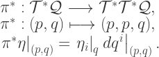
For the current purpose we will study the map

$\pi : \mathcal{T^*Q} \longrightarrow \mathcal{Q}, \:\:\:\:\:\:\:\: \pi(p, q) = q,$

that is, simply the projection map from $\mathcal{T^*Q}$ ‘down’ to $\mathcal{Q}$ – it just tells us the point on $\mathcal{Q}$ that the covector was living at.

Now for a mystical statement: the tautological 1-form is both the pullback $\pi^*$ interpreted as a 1-form, and also has the coordinate expression $\theta = p_i dq^i$ . How on earth can both these things be true, and besides, how can one ‘interpret a pullback as a 1-form’?!

That last claim is actually not too bad: a map $\mathcal{T^*Q} \longrightarrow \mathcal{Q}$ induces a pullback $\mathcal{T^*Q} \longrightarrow \mathcal{T^*T^*Q}$ , but this map has exactly the domain and range of a covector field on $\mathcal{T^*Q}$ ! Of course, this requires swapping between the perspectives of $p$ as a coordinate on $\mathcal{T^*Q}$ and $p$ as a 1-form in its own right.

We can use $(\eta,p,q)$ for coordinates on $\mathcal{T^*T^*Q}$ , equivalently writing $\eta = \eta^i dp_i + \eta_i dq^i$ where in a slight abuse of notation we’ve written $\eta^i$ for the first $n$ coordinates (the $dp$ components) and $\eta_i$ for the second $n$ coordinates (the $dq$ components).

Now to investigate $\pi$ and its induced pullbacks and pushforwards. Let $f : \mathcal{Q} \longrightarrow \mathbb{R}$ be a function on $\mathcal{Q}$ , and let $X : \mathcal{T^*Q} \longrightarrow \mathcal{TT^*Q}$ be a vector field on $\mathcal{T^*Q}$ , which in coordinates (using the same abuse of notation as before) we will write $X = X_i \partial_{p_i} + X^i \partial_{q^i}$ .

Recalling $\pi(p,q) = q$ , the pushforward of $X$ under $\pi$ is then

$\left.(\pi_* X)(f)\right|_{\pi(p,q)} = \left.X(f(\pi(p,q)))\right|_{(p,q)} \\ = \underbrace{\left.X_i \partial_{p_i}(f(q))\right|_{(p,q)}}_{=0} + \left.X^i \partial_{q_i}(f(q))\right|_{(p,q)},$

so the coordinates of our pushed-forward vector field on $\mathcal{TQ}$ are $(\pi_* X)^i = X^i$ , i.e. just the $q$ components of $X$ .

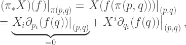
Now we can look at how $\pi^*$ acts on covector fields $\eta : \mathcal{Q} \longrightarrow \mathcal{T^*Q}$ (in coordinates $\eta = \eta_i dq^i$ ):

$\left.(\pi^* \eta)(X)\right|_{(p,q)} = \left.\eta(\pi_* X)\right|_{\pi(p,q)} \\ = \left.\eta_i dq^i\right|_q \left(\left.X^j \partial_{q^j}\right|_{(p,q)}\right) = \left.\eta_i\right|_q\left.X^i\right|_{(p,q)}.$

This means that the action of $\pi_*$ is basically to place $\eta$ straight into $\mathcal{T^*T^*Q}$ unchanged, with all $dp$ components set to zero:

$\pi^* : \mathcal{T^*Q} \longrightarrow \mathcal{T^*T^*Q}, \\ \pi^* : (p,q) \longmapsto (p, p, q), \\ \left.\pi^*\eta\right|_{(p,q)} = \left.\eta_i\right|_q \left.dq^i\right|_{(p,q)}.$

And this is the source of the coordinate expression for $\pi^*$ that I quoted above – it means that if we take $\pi^*$ to be a covector field on $\mathcal{T^*Q}$ , denoted $\theta$ , then

$\left.\theta\right|_{(p,q)} = \left.p_i\right|_q \left.dq^i\right|_{(p,q)},$

or $\theta = p_i dq^i$ for short. If you like you can think of the action of $\pi^*$ as stripping off the $dq$ components that belong to $\mathcal{T^*Q}$ and replacing them with $dq$ components that belong to $\mathcal{T^*T^*Q}$ .

How does it ‘cancel’ pullbacks?

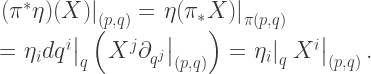
Now look at a general covector field $\alpha : \mathcal{Q} \longrightarrow \mathcal{T^*Q}$ . Treating $\alpha$ as a map (a similar trick to above) means it induces a pushforward $\alpha_* : \mathcal{TQ} \longrightarrow \mathcal{TT^*Q}$ and a pullback $\alpha^* : \mathcal{T^*T^*Q} \longrightarrow \mathcal{T^*Q}$ .

Let $F : \mathcal{T^*Q} \longrightarrow \mathbb{R}$ be a function, and $Y : \mathcal{Q} \longrightarrow \mathcal{TQ}$ a vector field with coordinate expression $Y = Y^i \partial_{q^i}$ , which is pushed-forward like so:

$(\alpha_* Y)(F) = Y(\alpha F) = Y^i \partial_{q^i} (F(\alpha, q)) \\ = \underbrace{Y^i \frac{\partial F}{\partial p_j} \left. \frac{\partial p_j}{\partial q^i} \right|_{p = \alpha}}_{=0} + Y^i \frac{\partial F}{\partial q_j} \left. \frac{\partial q_j}{\partial q^i} \right|_{p = \alpha} = \left. Y^i \right|_q \left. \partial_{q^i} F(p,q) \right|_{(\alpha, q)}.$

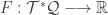
We can use this to find how $\alpha^*$ acts on covector fields $\beta : \mathcal{T^*Q} \longrightarrow \mathcal{T^*T^*Q}$ :

$\left. (\alpha^* \beta)(Y) \right|_q = \left. \beta(\alpha_* Y) \right|_{(\alpha,q)} = \left. \beta_i \right|_{(\alpha,q)} \left. Y^i \right|_q.$

But what if we specialise to $\beta = \theta = p_i dq^i$ , the interesting 1-form we were looking at above? We get

$\left. \alpha^* \theta \right|_q = \left. p_i dq^i \right|_{(\alpha,q)} = \left. \alpha_i dq^i \right|_q = \left. \alpha \right|_q,$

which is exactly the 1-form $\alpha$ that we started off with! This is the reason that $\theta$ is said to ‘cancel’ a pullback, as it gives us back the 1-form that we were using to create the pullback in the first place.

The basics of mechanics

How does this all link into physics? For mechanics you need a symplectic manifold $\mathcal{M}$ along with an 2-form called $\omega$ that satisfies various properties; notably that $d\omega = 0$ , so that at least locally we can find an $\alpha$ such that $d\alpha = \omega$ . Abstractly, we want to find paths $\Gamma : \mathbb{R} \longrightarrow \mathcal{M}$ such that the action integral $I$ is minimised:

$I(\Gamma) \equiv \int_\Gamma \alpha.$

Now, there are various ways to come up with symplectic manifolds, but the relevant one for physicists is ‘phase space’, i.e. $\mathcal{M} = \mathcal{T^*Q}$ , the cotangent bundle of some manifold $\mathcal{Q}$ (where we think of $\mathcal{Q}$ as being the ‘real’ physical space that we see around us, perhaps 4D space-time or similar). And it turns out that the logical choice of $\omega$ is to take $\omega \equiv -d\theta$ (the minus sign being a mere convention) where $\theta = p_i dq^i$ . Thanks to the discussion above we now know exactly what this object is (spoiler: it’s the tautological 1-form!).

Traditionally a physicist would have something called an action functional $S$ that takes curves $\gamma : \mathbb{R} \longrightarrow \mathcal{Q}$ and gives a real number, and they would then find the curve $\gamma$ that minimises that number ( $S$ is called a functional because it also depends on the first derivatives of $\gamma$ ). By parametrising $\gamma$ by the time coordinate the normal Euler-Lagrange equations are derived. However, we wish to stay agnostic about which coordinate represents time! So we will keep our paths parametrised by arc length, i.e. $\gamma : [0,1] \longrightarrow \mathcal{Q}$ .

Let $\gamma_q$ be a class of curves in $\mathcal{Q}$ parametrised by arc length with fixed starting point $\gamma_q(0) = q_0$ and ending point $\gamma_q(1) = q$ . Now define $W(q) \equiv S[\gamma_q] + W_0$ for some constant $W_0 \equiv W(q_0)$ , where $\gamma_q$ is defined to be the curve with endpoints $(q_0,q)$ that minimises $S[\gamma_q]$ . This function $W : \mathcal{Q} \longrightarrow \mathbb{R}$ is called Hamilton’s principal function, and note that it depends only on positions, and not the momenta! We now calculate

$S[\gamma_q] = W(q) - W(q_0) \\ \:\:\:\: = \int_{\partial \gamma_q} W \\ \ \:\:\:\: = \int_{\gamma_q} dW \:\:\:\:\:\:\:\: (1) \\ \ \:\:\:\: = \int_{\gamma_q} (dW)^* \theta \:\:\:\:\:\:\:\: (2) \\ \ \:\:\:\: = \int_{dW(\gamma_q)} \theta \:\:\:\:\:\:\:\: (3) \\ \ \:\:\:\: = \int_\Gamma \theta.$

The numbering refers to the following results:

Generalised Stokes’ theorem. Here the ‘boundary’ of $\gamma_q$ is just its two endpoints.
The ‘cancelling’ property described above: $\eta^*(\theta) = \eta$
A standard property of integrals of pullbacks: $\int_U \Phi^*(\eta) = \int_{\Phi(U)} \eta$

So we see that the process of minimising $S$ is just a special case of the general theory of minimisation problems on symplectic manifolds. To lift the path $\gamma$ from $\mathcal{Q}$ to the symplectic phase space $\mathcal{T^*Q}$ , we used the 1-form $dW$ as a pullback, similarly to the trick we pulled above with $\pi^*$ . That means that the momenta along $\gamma$ are

$p_i = \frac{\partial W}{\partial q^i}.$

Ignoring any details of the expression for the action $S$ , how do we derive a more familiar set of differential equations that determine $\gamma$ ? We can pick out one of the coordinates, say $q^0$ , and call it time $t$ , and similarly one of the momenta, say $p_0$ , and call it energy $-H$ (again, minus sign by convention), so that

$H = -\frac{\partial W}{\partial t}.$

Our aim is to eliminate $W$ in favour of the other coordinates (we will still write $q^i$ and $p_i$ for the other (n-1) coordinates).

Recall that $d^2W = 0$ by the definition of the exterior derivative, so we can immediately write down the first of Hamilton’s equations:

$\frac{\partial}{\partial t}\left(\frac{\partial W}{\partial q^i}\right) = \frac{\partial}{\partial q^i}\left(\frac{\partial W}{\partial t}\right) \\ \frac{\partial p_i}{\partial t} = -\frac{\partial H}{\partial q^i}.$

And since subtracting a total differential from $dW$ retains the $d^2 = 0$ property, we can define a quantity that gives us the second of Hamilton’s equations:

$dA \equiv dW - d(p_iq^i) \\ \frac{\partial}{\partial t}\left(\frac{\partial A}{\partial p_i}\right) = \frac{\partial}{\partial p_i}\left(\frac{\partial A}{\partial t}\right) \\ \frac{\partial q_i}{\partial t} = \frac{\partial H}{\partial p_i}.$

Note that we now have explicitly

$\theta = p_i dq^i - Hdt \\ \omega = dq^i \wedge dp_i - dt \wedge dH$

for our symplectic structure, and we ended up with the familiar Hamilton’s equations

$\frac{\partial p_i}{\partial t} = -\frac{\partial H}{\partial q^i} \\ \frac{\partial q_i}{\partial t} = \frac{\partial H}{\partial p_i}.$

And so, as if by magic, we’ve recovered the traditional formalism of Hamiltonian mechanics as a special case of minimisation procedures on symplectic manifolds.

Of course, we didn’t have to use the 0th coordinate to represent time/energy. Really, time and position are distinguished from each other by the form of the Lorentzian metric, which has not yet entered into our method. It’s true that non-relativistic mechanics will inevitably privilege a time variable; but, the action for a free relativistic point particle is nicely Lorentz-invariant:

$S[\gamma] = \int_\gamma \left.g(X,X)\right|_{\gamma(s)}ds$