The setting for dynamics is the cotangent bundle of a manifold with pseudo-Riemannian metric ; relevant observables can be functions of both position and momentum. For example, the distribution function , which is the number density of particles in phase space ( and are coordinates on and respectively).

The spatial volume form (integral measure) is , where is the determinant of the metric evaluated at ; and the volume form for the full phase space is . If we want to integrate out the momentum-dependence of some observable, we need just the momentum-part of the volume form. From the two expressions above we can see that this is .

However, paths that obey the classical equations of motion are constrained to lie on the mass-shell: in flat Lorentzian spacetime this is a hyperboloid in the momentum cotangent space , given by 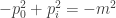, where is the energy, the spatial 3-momentum and m the rest mass of a particular particle. However, in fully general curved spacetime the corresponding condition gives a hypersurface .

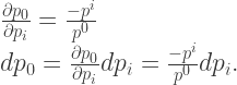
Because the permitted region of phase space has been restricted, we can eliminate one momentum component from the integral, treating it as a function of the other coordinates. Conventionally we pick to be this unwanted component, writing , and note that the equation for can be written 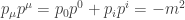, which allows us to solve for .

We then find the volume form induced on . Let be the unit vector field normal to :

The denominator works out to be . Noting that the metric is a function of alone, we perform the derivative on the numerator and so find that

(the normal index convention for vectors and covectors is swapped round, as we are working on , so the coordinates are covariant to begin with).

In general, the volume form induced from a manifold onto a submanifold with normal VF is

For the present purposes we therefore have

We differentiate the condition with respect to a spatial component and rearrange, giving (note the positions of the indices):

Expressions of the form 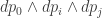can be simplified to involve only the -component of ( ), as repetition of a form in a wedge product sets the entire expression to zero. We also have .

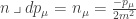So, putting it all together,

And so the final result is

which has the expected form. Integrals over momentum space therefore look like

Everything we wrote down was manifestly covariant, so this volume form transforms in the correct way under general coordinate transformations. The rest mass does not appear in the final volume form, so we are free to set if we choose, as is the case with photons.