Cheap & Easy differential forms

There’s a way of motivating the notions of tangent vectors and covectors that’s hinted at but generally glossed over – at least in the physics courses that I take. This post is a quick overview, serving mostly as a reminder to myself of the topic. Please excuse the lack of rigour.

I will use the Einstein summation convention throughout,

$x^iy_iz^j \equiv \sum\limits_i \: x^iy_iz^j,$

and hopefully by the end I’ll even have explained why it makes sense.

Tangent vectors

We have an $n$ -dimensional manifold $M$ , which contains points, but not vectors. You cannot subtract two points on a manifold and expect to get something useful; imagine a line drawn between two points on the Earth’s surface. It would go awkwardly underground, and wouldn’t measure any sort of quantity that’s appreciable by inhabitants on the surface.

Let $\gamma \: : \: \mathbb{R} \longrightarrow M$ be a curve on $M$ . It takes some real parameter (lets call it $t$ ) and spits out points in $M$ along a line, as you evolve $t$ . Let’s call the coordinates of these points $p^i(t)$ in some coordinate system, and $p'^i(t)$ in some other coordinate system. Then we can find a ‘velocity’ vector $\dot{\gamma}$ , tangent to the curve, whose coordinates are $\left(\frac{dp^1}{dt}, \frac{dp^2}{dt}, \ldots, \frac{dp^n}{dt}\right)$ . The coordinates of $\dot{\gamma}$ in the primed coordinate system are then given by the chain rule,

$\frac{dp'^i}{dt} = \frac{dp'^i}{dp^j}\frac{dp^j}{dt}.$

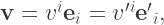
This motivates the study of all objects that transform this way, and they are called contravariant vectors, or contravectors, or just vectors.

Now, so far the vectors are just $n$ -tuples of numbers, with no particular geometric significance. I will however write down a vector $\mathbf{v}$ with a basis by pairing up its components $v^i$ with a basis $\mathbf{e}_i$ , as well as the same in the primed coordinate system:

$\mathbf{v} = v^i\mathbf{e}_i = v'^i\mathbf{e'}_i,$

and for now these basis vectors $\mathbf{e}_i$ are formal placeholders. All we can say is, whatever the choice of $\mathbf{e}_i$ , they will have to transform using the inverse of the transformation matrix used by $v^i$ , in order that the expression above remains true in any coordinate system.

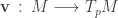
A vector lives at a single point $p$ of $M$ , in a space called ‘the tangent space to $M$ at $p$ ‘, or $T_pM$ for short – imagine a flat plane ( $T_pM$ ) balancing on top of a lumpy surface ( $M$ ), touching it at a point ( $p$ ). If $\mathbf{v}$ varies from point to point, it is strictly a vector field, or in other words a function $\mathbf{v} \: : \: M \longrightarrow T_pM$ ; in this case we can just say that it lives in $TM$ , and we have to be careful not to forget about its position-dependence even if we suppress it occasionally for notational convenience.

Differential operators

Let $f \: : \: M \longrightarrow \mathbb{R}$ be a scalar field (just a real-valued function) on our manifold $M$ . We can write differentiation of $f$ along a vector (the directional derivative along $\mathbf{v}$ ) in three ways, all defined to be equivalent

$\left( \nabla_\mathbf{v} f \right) (p) \equiv \frac{df(p + t\mathbf{v})}{dt}\Big|_{t = 0} \equiv v^i\frac{\partial f}{\partial x^i},$

and note that we’re not really adding the vector $\mathbf{v}$ to the point $p$ , because we’re evaluating the expression at $t = 0$ . The $p$ -dependence is casually suppressed in the last expression.

We might worry that this is coordinate system-dependent, so lets try to write the same quantity down in the primed coordinate system, using the transformation properties of $\mathbf{v}$ that we already know, and the chain rule:

$v'^i\frac{\partial f}{\partial x'^i} = \frac{\partial x'^i}{\partial x^j} v^j \frac{\partial f}{\partial x^k}\frac{\partial x^k}{\partial x'^i} = v^j \frac{\partial f}{\partial x^k} \delta^k_j = v^k \frac{\partial f}{\partial x^k},$

so our directional derivative is coordinate-invariant after all! Note that multiplying the coordinates of a matrix with those of its inverse (and summing according to the Einstein convention) gives the Kronecker delta, which is why we can swap out $j$ for $k$ in the last expression.

Coordinate-invariance shouldn’t surprise us too much, because the first two ways of writing the directional derivative made no mention of any coordinate system for $\mathbf{v}$ .

Now, recall that first-order differential operators on real functions of $n$ variables all take the form

$D f = a^i\frac{\partial f}{\partial x^i},$

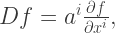
and so if we just interpret the values $a^i$ as components of a vector, we’ve found a one-to-one correspondence between vectors and first-order differential operators (strictly speaking it’s between vector components and operators, but all the transformation matrices between coordinate systems are one-to-one too so it doesn’t matter).

This correspondence with differential operators hints strongly at what quantities to use as our basis vectors – the individual derivative operators $\frac{\partial}{\partial x^i}$ certainly transform in the correct way. We now make the formal identification

$\frac{\partial}{\partial x^i} \equiv \mathbf{e}_i.$

I say formal because we will not treat these basis vectors like ‘proper’ derivative symbols, as their ‘true’ meaning will only come into play in certain carefully-defined situations.

Let’s make the following abbreviations: $\frac{\partial}{\partial x^i} \equiv \partial_i$ and $\frac{\partial}{\partial x'^i} \equiv \partial'_i$ when talking about operators; and $\frac{\mathbf{\partial}}{\mathbf{\partial} x^i} \equiv \partial_i \equiv \mathbf{e}_i$ and $\frac{\mathbf{\partial}}{\mathbf{\partial} x'^i} \equiv \partial'_i \equiv \mathbf{e'}_i$ when talking about basis vectors.

Linear functionals

A linear functional is a function $\alpha \: : \: TM \longrightarrow \mathbb{R}$ that satisfies linearity, i.e.

$\alpha(\mathbf{u}) = x \in \mathbb{R} \\ (\alpha + \beta)(\mathbf{u}) = \alpha(\mathbf{u}) + \beta(\mathbf{u}) \\ \alpha(\mathbf{u} + \mathbf{v}) = \alpha(\mathbf{u}) + \alpha(\mathbf{v}).$

Linear functionals are ‘vector-like’, but live in a space called $T^*M$ , rather than the $TM$ that contains vectors. They are totally determined by their action on the basis vectors of $TM$ , so can be written down in components:

$\alpha_i = \alpha(\mathbf{e}_i) \\ \alpha(\mathbf{v}) = \alpha_i v^i \\ \alpha = \alpha_i\eta^i \\ \eta^i(\mathbf{v}) = v^i,$

where the $\eta^i$ are some as-yet-mysterious basis for our linear functionals. Note the position of the indices on each quantity: the Einstein summation convention is working correctly, even if we don’t necessarily know yet what sort of quantities we’re dealing with.

The expression $\alpha(\mathbf{v}) = \alpha_i v^i$ must be coordinate independent, as the left hand side makes no reference to any coordinate system; and we already know how to transform $v^i$ . Therefore the components $\alpha_i$ must use the opposite transformation, $\alpha'_i = \alpha_j \frac{\partial x^j}{\partial x'^i}$ . So we have

$\alpha'_i v'^i = \alpha_j \frac{\partial x^j}{\partial x'^i} \frac{\partial x'^i}{\partial x^k} v^k = \alpha_j \delta^j_k v^k = \alpha_j v^j = \alpha(\mathbf{v}).$

These linear functionals are also called covariant vectors, covectors, differential one-forms, or one-forms. Remember that both $\alpha$ and $\mathbf{v}$ can have $p$ -dependence in general, making them covector fields and vector fields respectively.

Total differential of a function

The following formula for the ‘total’ differential of a function should be familiar:

$df = \partial_i f dx^i,$

where $p$ -dependence has been suppressed on both sides. However, we don’t currently have a way to make geometric sense of the individual coordinate differentials $dx^i$ . This expression must be coordinate-independent (no mention of coordinates is made on the left side), so the coordinate differentials must transform as

$dx'^i = \frac{\partial x'^i}{\partial x^j} dx^j.$

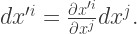
This is exactly how the basis for our covectors $\eta^i$ transforms! So we can make the formal identification $\eta^i \equiv dx^i$ , much like how we earlier decided that $\mathbf{e}_i \equiv \partial_i$ .

The full component-wise expression for the action of our covectors on our vectors is

$\alpha(\mathbf{v}) = \alpha_i v^j dx^i(\partial_j) = \alpha_i v^j \delta^i_j = \alpha_i v^i.$

The only trick here is $dx^i(\partial_j) = \delta^i_j$ , which we have defined to be true.

Our expression for $df$ now comes in handy as a way to generate new covectors. In fact, covectors generated in this way have the following useful property:

$df(\mathbf{v}) = \partial_i f v^i = \nabla_\mathbf{v} f.$

You may have spotted by now the value of the Einstein summation convention – as long as you keep your up-indices on vector components (and covector bases), and down-indices on covector components (and vector bases), any scalar you end up with will be coordinate-independent. This is a useful ‘type-check’ on any expression; if the indices don’t match, something must be wrong (or you’ve violated relativity by finding a preferred coordinate system).

I finish with three warnings:

Covectors generated from functions (like $df$ above) are not the only kind! Any linear combination of the basis covectors $dx^i$ is a covector, and in general the arbitrary covector $a_i dx^i$ will not be the differential of any function at all.
The components of vectors transform in the opposite way to the components of covectors. The basis vectors transform oppositely to the vector components, and to the basis covectors. This is confusing! Hence physicists like to pretend that basis vectors don’t exist, and only work with components. This is a convenient way to work for many computations, but you can end up getting confused when your basis vectors change from point-to-point (as they do on most non-trivial manifolds and coordinate systems):
$\frac{d\mathbf{v}}{dt} = \frac{d}{dt}\left(v^i \mathbf{e}_i\right) = \dot{v}^i\mathbf{e}_i + v^i\mathbf{\dot{e}}_i.$

Mathematicians never write any down coordinates, say they are working in a ‘coordinate-free’ way, and act all clever about it.
There is one more way to write the directional derivative, which is
$\mathbf{v}\left(df\right) = v^i \frac{\partial f}{\partial x^j} \partial_i(dx^j) = v^i \frac{\partial f}{\partial x^j} \delta^j_i = v^i \frac{\partial f}{\partial x^i} = \nabla_\mathbf{v} f,$

treating $\mathbf{v}$ as a function $T^*M \longrightarrow \mathbb{R}$ . Unfortunately you also see people write the above as

$\mathbf{v}\left(f\right) = v^i \partial_i f = \nabla_\mathbf{v} f,$

which is very confusing, as it conflicts with our careful definitions of what the basis vectors and covectors mean – such is life.